Data Flow
- Discover a lidar measurement with
lidarpy.utils.file_manager. - Convert Licel binary files to NetCDF with
lidarpy.nc_convert.measurement. - Run preprocessing with
lidarpy.preprocessing.preprocess. - Inspect products with
lidarpy.plot.quicklook. - Use synthetic signals to validate retrieval behavior independently from RAW fixtures.
- Run ABLH detection on normalized lidarpy or Cloudnet ceilometer products.
- Use SCC support modules only when the external SCC environment is explicitly available.
Stage 1: RAW Discovery and NetCDF Conversion
RAW fixtures are intentionally small in this repository, but the code path mirrors production use: locate a measurement, unzip/read Licel files, map channels through system configuration and write NetCDF. This stage is tested because every downstream correction depends on stable dimensions, coordinates and metadata.
| Input | Primary code | Expected product |
|---|---|---|
| ALHAMBRA RAW RS/DC zip fixtures | lidarpy.nc_convert.measurement.Measurement |
One NetCDF file per converted measurement. |
| System TOML/YAML package data | lidarpy.nc_convert.configs and lidarpy.info |
Channel metadata, bin-zero values and lidar system attributes. |
| ACTRIS/SCC parameter resources | Measurement.scc_config_id and lidarpy.scc.utils |
Detected SCC configuration ID from Licel header channels and actris_config.yml rules. |
Stage 2: Preprocessing
Corrections are ordered so that each step sees a physically meaningful signal. Dark-current correction comes before dead-time and background handling; bin-zero shifts are applied before overlap correction; cropping and smoothing happen after range-dependent corrections.
apply_dc: subtract dark current where a matching DC measurement is available.apply_dt: correct photon-counting dead time.apply_bg: remove background from a far-range interval.apply_bz: shift signals using channel bin-zero metadata.apply_ov: apply overlap from a file or derive it from full-field/near-field channels.gluing_products: merge analog and photon-counting products where configured.apply_sm: smooth the final corrected product.
The migrated ALHAMBRA tests cover the basic corrections, generated
overlap files, derived overlap from 1064fta/1064nta
and near-field 532 nm gluing products.
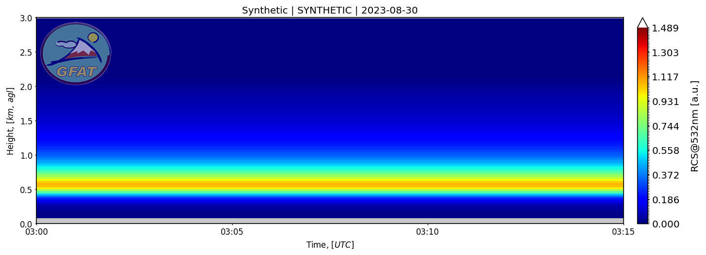
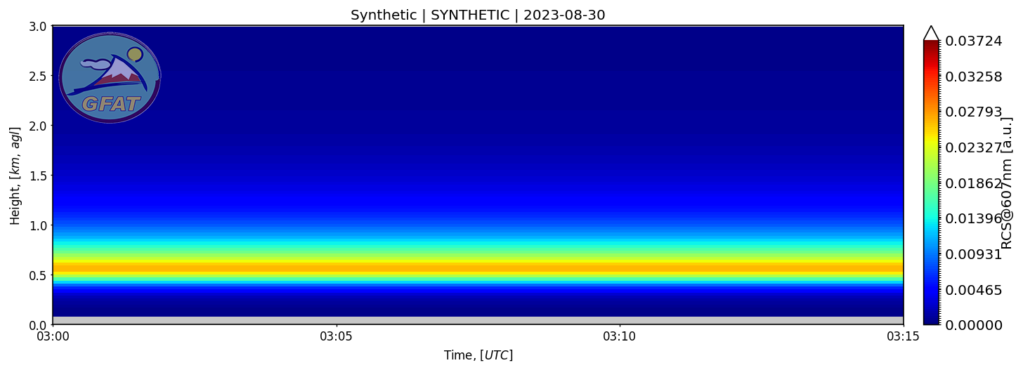
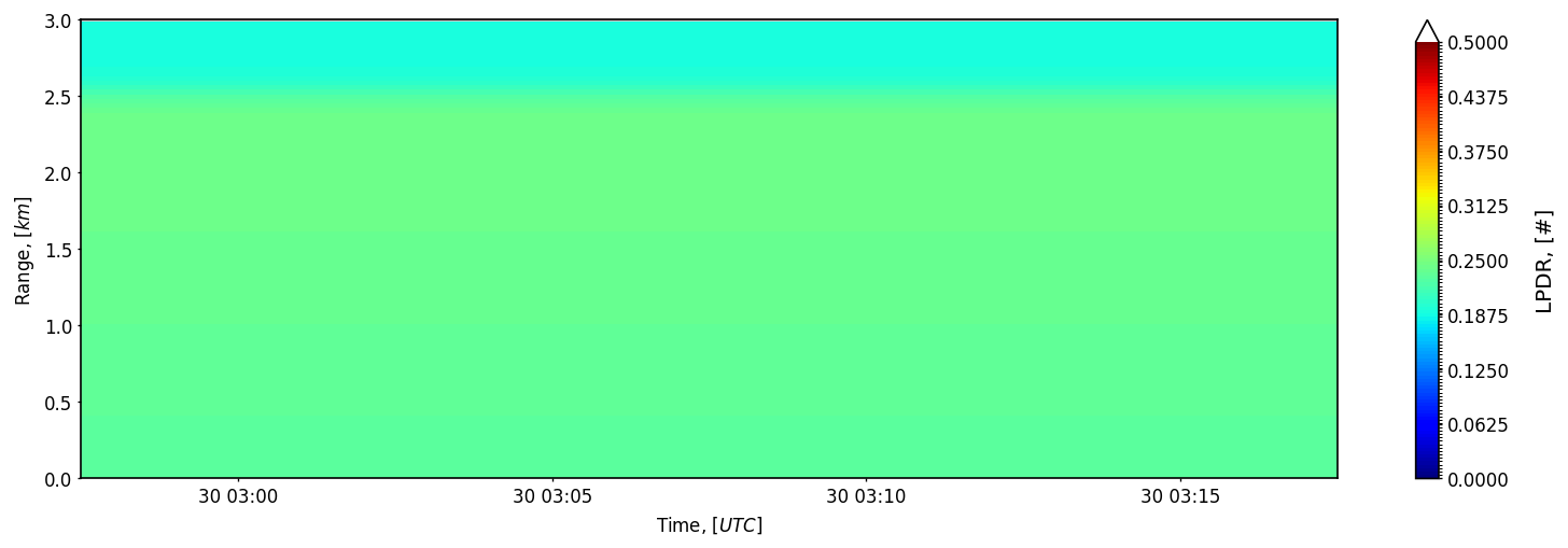
Stage 3: Plotting and Inspection
Quicklooks are operational diagnostics. A successful quicklook confirms that a product has the expected dimensions, coordinates and signal naming contract. It does not prove scientific quality by itself, but it catches many data-shape failures that are hard to notice in arrays.
Stage 4: Retrieval Validation
Retrieval validation uses synthetic truth because RAW measurements rarely provide exact aerosol profiles. The goal is not to make every retrieval exact everywhere; it is to compare in a range where the assumptions are explicit and the boundary conditions are valid.
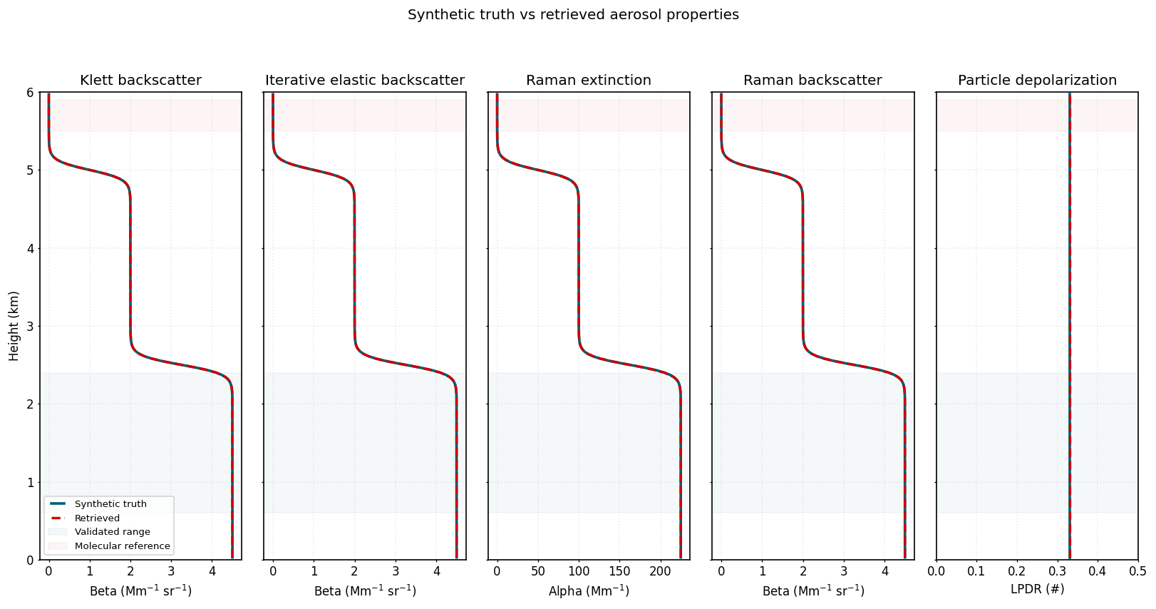
quasi_betais tested as a single-iteration approximation.iterative_beta_forwardcan start above the first range bin wheninitial_particle_optical_depthis known.- Reference intervals outside the profile raise
ValueError. - Klett, Raman extinction and Raman backscatter are compared outside near-field and boundary regions.
Stage 5: ABLH Products
ABLH detection is exposed through lidarpy.retrieval.ablh.
The adapter accepts lidarpy datasets containing signal_*
variables and Cloudnet ceilometer datasets containing
beta_smooth, beta or beta_raw.
Lidarpy signals are range-corrected before detection; Cloudnet
backscatter is used directly.
The detector returns a small NetCDF-ready dataset with
ablh, ablh_range and
ablh_height. For Cloudnet inputs, ablh_height
is interpolated from the product height coordinate so users can preserve
both height above instrument and height above mean sea level.
| Method | Use | Main tunables |
|---|---|---|
wct |
Haar wavelet covariance transform for strong negative gradients. | wct_width, threshold, search range. |
temporal_variance |
Strong temporal variance layer in a moving time window. | time_window_minutes, threshold, search range. |
Operational States
| State | How to recognize it | Next action |
|---|---|---|
| RAW converted | NetCDF exists and has time, range and channel. |
Run a narrow preprocessing test or inspect with xarray. |
| Preprocessed | Dataset attrs show correction flags such as bg_corrected and ov_corrected. |
Generate or inspect quicklooks. |
| Validated by synthetic truth | Focused retrieval tests pass in the expected comparison range. | Use the algorithm with measured data and document assumptions. |
| SCC ready offline | SCC package data and mocked access-client tests pass. | Use real SCC credentials only in an explicit external environment. |